Spectral Sheaves

This post is based on my thesis proposal presentation.

Introduction

My research plan stems from a very simple observation: whenever you have a coboundary operator acting on a finite-dimensional vector space, you can define a Laplacian. The traditional manifestation of this fact is the graph Laplacian, the source of so much joy in spectral graph theory. There we consider the coboundary operator \(\delta: \mathbb{R}^V \to \mathbb{R}^E\) and form the Laplacian \(L = \delta^* \delta\). The spectrum of \(L\) can tell you a lot about the graph.

But there’s another simple situation where we have a coboundary operator: a sheaf on a graph. A sheaf \(\mathcal{F}\) on a graph \(G\) is an assignment of a vector space \(\mathcal{F}(v)\) to each vertex \(v\), a vector space \(\mathcal{F}(e)\) to each edge \(e\), and a map \(\rho_{ve}: \mathcal{F}(v) \to \mathcal{F}(e)\) for each incident edge-vertex pair \(v \leq e\). The vector spaces \(\mathcal{F}(v)\) and \(\mathcal{F}(e)\) are called stalks over \(v\) and \(e\), and the map \(\rho_{ve}\) is called a restriction map. We get two vector spaces of cochains, \(C^0(G;\mathcal{F}) = \bigoplus_{v \in V} \mathcal{F}(v)\), and \(C^1(G;\mathcal{F}) = \bigoplus_{e \in E} \mathcal{F}(e)\). Assigning an orientation to the edges of \(G\) gives us an incidence number \(i(v,e) \in \{\pm 1\}\) depending on whether the edge is oriented toward or away from the vertex. This lets us define a coboundary operator \(\delta: C^0(G;\mathcal{F}) \to C^1(G;\mathcal{F})\) by \(\delta(x) = \sum_{v \in V} \sum_{v \leq e} i(v,e) \rho_{ve} x|_{\mathcal{F}(v)}\).

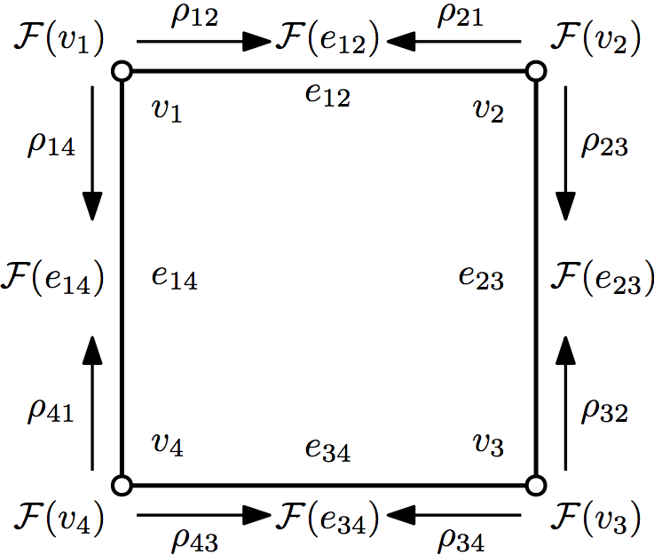
How should we think about a sheaf on a graph? We can assign local data to each vertex. The restriction maps tell us when an assignment of data is globally consistent. So a sheaf mediates the passage from collections of local information to a global picture. We call an assignment of data to each \(\mathcal{F}(v)\) that is consistent over the edges a global section. That is, \(x \in C^0(G;\mathcal{F})\) is a global section if \(\rho_{ve} x|_{\mathcal{F}(v)} = \rho_{v'e} x|_{\mathcal{F}(v')}\) for all edges \(e = (v,v')\). A moment of consideration will show that \(x\) is a global section precisely when \(\delta x = 0\).

We now have a coboundary operator and want to construct its associated Laplacian. To do this, we need one more piece of information: an inner product on each stalk \(\mathcal{F}(v)\) and \(\mathcal{F}(e)\) allows us to identify these spaces with their duals and take the adjoint \(\delta^*\) of \(\delta\). Then we define \(L_{\mathcal{F}} = \delta^ \delta\) as before. A standard result from linear algebra says that \(\ker L = \ker \delta\), and further, \(\langle x,Lx \rangle = \langle \delta x, \delta x \rangle = \lVert\delta x\rVert^2 \geq 0\), so \(L\) is positive semidefinite.

I’m not the first one to make these observations. Joel Friedman proved the Hanna Neumann conjecture using something he called sheaves on graphs. (Under our definitions, these would be cosheaves on graphs—-the maps go the opposite direction.) As an aside in the introduction of this paper, he suggested defining Laplacian and adjacency matrices for sheaves and studying their spectral properties. Others have worked with special cases of the sheaf Laplacian, most notably the work by Singer and various others on the graph connection Laplacian, which is the Laplacian of a sheaf all of whose restriction maps are in \(O(n)\).

Results

Eigenvalue interlacing

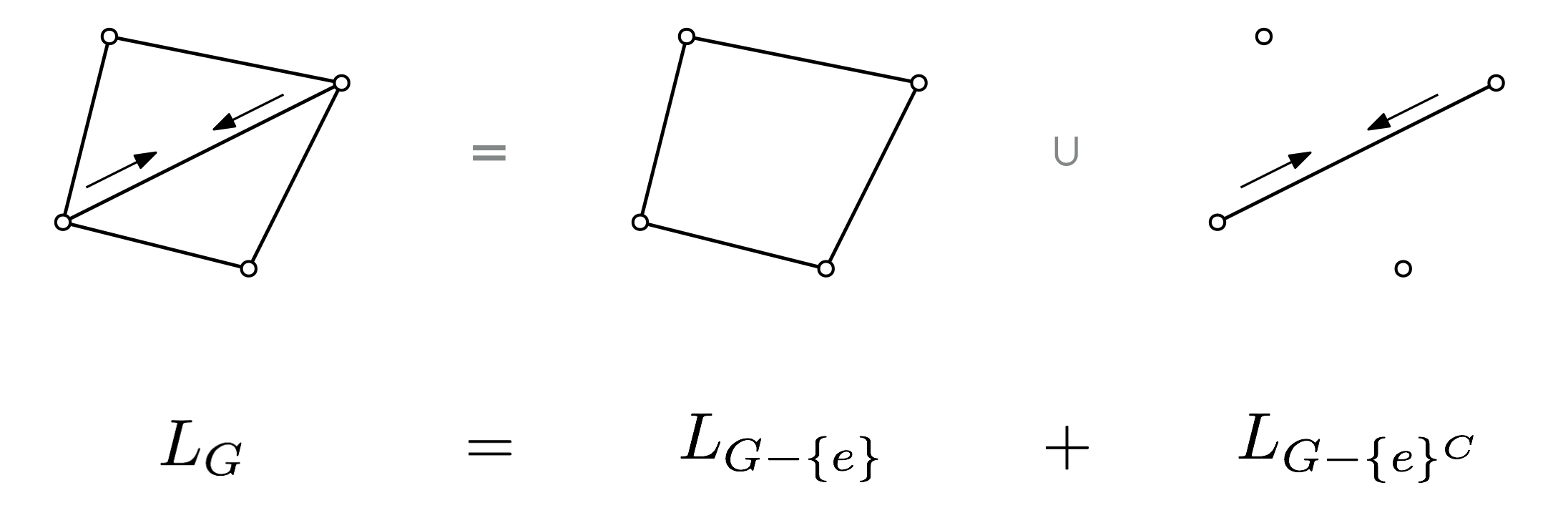
One of the first questions you might ask about graph spectra is what happens to the spectrum of a graph when you remove an edge. It’s natural to ask the same question about a sheaf on a graph. The way to get the required information is to look at the Laplacian of the larger graph as the sum of two Laplacians: one corresponding to the smaller graph, and one corresponding to the removed edge. To understand how the spectra are related, we define a notion of interlacing:

Let \(A\), \(B\) be \(n \times n\) matrices with real spectra, and let \(\lambda_1\leq \lambda_2 \leq \cdots \leq \lambda_n\) be the eigenvalues of \(A\) and \(\mu_1 \leq \mu_2 \leq \cdots \leq \mu_n\) be the eigenvalues of \(B\). We say the eigenvalues of \(A\) are \((p,q)\)-interlaced with the eigenvalues of \(B\) if for all \(k\), \(\lambda_{k-p} \leq \mu_k \leq \lambda_{k+q}\). (We let \(\lambda_{k} = \lambda_1\) for \(k \lt 1\) and \(\lambda_k = \lambda_n\) for \(k \gt n\).)

We now show that the eigenvalues of sheaf Laplacians are interlaced after deleting a subgraph. Let \(\mathcal{F}\) be a sheaf on a graph \(G\), and let \(C\) be a collection of edges of \(G\), and denote \(H = G\setminus C\) to be \(G\) with the edges in \(C\) removed. Let \(L_G\) be the sheaf Laplacian of \(\mathcal{F}\) and \(L_H\) the sheaf Laplacian of \(i^* \mathcal{F}\). Define further the sheaf \(\mathcal G\) to be the sheaf with the same vertex stalks as \(\mathcal{F}\) but with all edge stalks over edges not in \(C\) set to zero. Then we have the following:

Proposition

The eigenvalues of \(L_H\) are \((t,0)\)-interlaced with the eigenvalues of \(L_G\), where \(t = \text{codim} H^0(G;\mathcal G) = \dim C^0(G; \mathcal{F}) - \dim H^0(G;\mathcal G)\).

Proof. Notice that \(L_H = L_G - L_C\), where \(L_C\) is the Laplacian of \(\mathcal G\). By the Courant-Fischer theorem, we have

\[\mu_k = \min_{\dim Y = k} \left(\max_{y \in Y,y\neq 0} \frac{\langle y,L_G y \rangle - \langle y, L_Cy \rangle}{\langle y, y \rangle}\right)\] \[\hphantom{\mu_k } \geq \min_{\dim Y = k} \left(\max_{y \in Y \cap H^0(G;\mathcal G),y\neq 0} \frac{\langle y,L_G y \rangle}{\langle y, y \rangle}\right)\] \[\hphantom{\mu_k } \geq \min_{\dim Y = k - t } \left(\max_{y \in Y,y\neq 0} \frac{\langle y,L_G y \rangle}{\langle y, y \rangle}\right) = \lambda_{k-t}\]

and

\[\lambda_k = \min_{\dim Y = k} \left(\max_{y \in Y,y\neq 0} \frac{\langle y,L_G y \rangle}{\langle y, y \rangle}\right)\] \[\hphantom{\lambda_k } \geq \min_{\dim Y = k} \left(\max_{y \in Y,y\neq 0} \frac{\langle y,L_G y \rangle - \langle y, L_Cy \rangle}{\langle y, y \rangle}\right) = \mu_{k}\]

Pullbacks and covering maps

If you have a morphism \(f: H \to G\) of graphs, a sheaf \(\mathcal{F}\) on \(G\) can be turned into a sheaf \(f^*\mathcal{F}\) on \(H\) by letting \(f^*\mathcal{F}(v) = \mathcal{F}(f(v))\), \(f^*\mathcal{F}(e) = \mathcal{F}(f(e))\), and \(\rho_{ve}: f^*\mathcal{F}(v) \to f^*\mathcal{F}(e)\) be equal to \(\rho_{f(v)f(e)}\). This is known as the pullback sheaf. There is a natural map \(f^*: C^i(G;\mathcal{F}) \to C^i(H;f^*\mathcal{F})\) whose definition you can probably figure out faster than I can type it. This map is nice in that \(\delta f^* = f^* \delta\); in particular this means that every section of \(\mathcal{F}\) lifts to a section of \(f^*\mathcal{F}\). Anyone familiar with cohomology should not be surprised by this fact: it is essentially the fact that cohomology is a contravariant functor. On the other hand, \(f^*\) does not commute with \(\delta^*\) in general. But if \(f\) is a covering map, it does!

Lemma

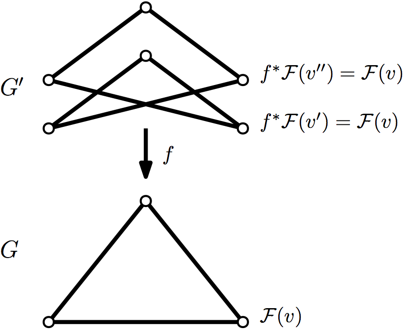
Suppose \(f: H \to G\) is a covering map of graphs; that is, for any vertex \(v \in H\), \(f\) is an isomorphism of graphs when restricted onto the neighborhood of \(v\). Then \(\delta^*_{f^*\mathcal{F}} = f^* \delta^*_{\mathcal{F}}\).

Proof. For \(y \in C^0(H;\mathbb{F}^*\mathcal{F})\) and \(x \in C^{1}(G;\mathcal{F})\), we have \(\langle y,\delta^*f^*x \rangle = \langle \delta y, f^*x \rangle = \sum_{v' \leq e'} i({v',e'}) \langle \rho_{v' e'}(y_{v'}), (f^* x)_{e'} \rangle = \sum_{v' \leq f(e)} i({v', f(e)}) \langle \rho_{v' f(e)}(y_{v'}),x_\tau \rangle\) \(= \sum_{v \leq e} i(v, e) \sum_{v' \in f^{-1}(v)} \langle \rho_{v e}(y_{v'}),x_e \rangle = \sum_{v \leq e} i(v, e) \langle \rho_{v e} ((f^*)^*y)_v,x_e \rangle = \langle \delta (f^*)^* y, x \rangle = \langle y,f^* \delta^* x \rangle.\)

The first equality is by definition of the adjoint, the second the definition of the coboundary map, the third the definition of \(f^*\), and the fourth equality holds because \(f\) is a covering map. The fifth equality comes from computing the adjoint of \(f^*\), the sixth from the definition of \(\delta\), and the last again from the definition of adjoints.

The key point is that every vertex in \(H\) maps down to a vertex whose neighborhood looks exactly the same.

The fact that \(\delta^*\) commutes with \(f^*\) means we can say a lot about the spectrum of \(f^*\mathcal{F}\). In particular, we know that if \(L_{\mathcal{F}} x = \lambda x\), then \(L_{f^*\mathcal{F}} f^* x = \delta^*_{f^*\mathcal{F}}\delta_{f^*\mathcal{F}} f^* x = f^* \delta^*_{\mathcal{F}}\delta_{\mathcal{F}} x = f^* L_{\mathcal{F}} x = \lambda f^*x\), so \(x\) is an eigenvector of \(L_{f^*\mathcal{F}}\) with eigenvalue \(\lambda\). So the spectrum of \(\mathcal{F}\) is contained in the spectrum of \(f^*\mathcal{F}\). So we have

Theorem

If \(H \to G\) is a covering map of graphs, with \(\mathcal{F}\) a sheaf on \(G\), then \(\sigma(f^*\mathcal{F}) \supseteq \sigma(\mathcal{F})\).

Harmonic functions

Harmonic functions are perhaps most familiar from analysis, where they share many nice properties with holomorphic functions. One of these is an averaging property: the value of a harmonic function at a point is equal to the average value of the function on a sphere centered at the point. Another is the maximum principle: a function which is harmonic on some compact set attains its maximum on the boundary of the set. We can define an analogous condition for functions on graphs: a function \(f\) is harmonic at a vertex \(v\) if \(Lf(v) = 0\). Equivalently, the value of \(f\) at \(v\) is equal to the (weighted) average of the value of \(f\) at neighbors of \(v\). This definition generalizes immediately to sheaves, and we note that the functions which are everywhere harmonic are precisely the global sections of the sheaf.

Harmonic functions on graphs also satisfy a maximum principle: a function on a graph which is harmonic away from some boundary set \(B\), where every vertex in \(B\) is connected to the rest of the graph, attains its maximum value on \(B\). There is a further extension to sheaves whose restriction maps are all in the orthogonal group \(O(n)\): a 0-cochain which is harmonic away from a set \(B\) attains its maximum pointwise norm on \(B\). To be precise, we have:

Proposition

Let \(\mathcal{F}\) be an a weighted sheaf on a graph \(G\) with all restriction maps in \(O(n)\). Suppose \(f \in C^0(G;\mathcal{F})\), and that \(f\) is harmonic on a subset of vertices \(H \subseteq G\). Further suppose that the subgraph induced by \(H\) is connected, and that every vertex of \(G \setminus H\) is connected to \(H\). Then if \(f\) attains its maximum norm on \(H\), its vertexwise \(\ell^2\) norm is constant.

Proof. Let \(v \in H\) and suppose \(\lVert f(v)\rVert \geq \lVert f(w)\rVert\) for all \(w \in G\). Then because \(f\) is harmonic at \(v\), \(\lVert f(v)\rVert = \frac{1}{d_v} \lVert\sum_{w \sim v} \rho_{vw}f(w)\rVert \leq \frac{1}{d_v} \sum_{w \sim v} \lVert\rho_{vw}f(w)\rVert = \frac{1}{d_v} \sum_{w \sim v} \lVert f(w)\rVert \leq \frac{1}{d_v} \sum_{w \sim v} \lVert f(v)\rVert = \lVert f(v)\rVert.\)

Therefore, equality holds throughout, so \(\lVert f(v')\rVert = \lVert f(v)\rVert\) for any \(v' \sim v\). But by hypothesis, every vertex in \(H\) is connected via a path lying in \(H\) to \(v\), so we can repeat this argument to show that \(\lVert f(v)\rVert\) is constant for all \(v \in H\). But now this argument shows that \(f\) is also constant for every \(v \notin H\).

Sparsification

Graphs can be complicated; a graph on \(n\) vertices can have \(O(n^2)\) edges. Often, it would be nice if we could replace a graph that has many edges with one that has relatively fewer. Of course, we want the smaller graph to share important properties with the original graph. One way to measure this similarity is using the Laplacian spectrum of the graph. Given two symmetric matrices \(A\), \(B\), we say that \(A \preceq B\) if \(B-A\) is positive semidefinite. This imposes a relationship between both the eigenvalues and eigenvectors of \(B\) and \(A\).

Spielman and Teng give a sparsification result for weighted graphs:

Theorem (Spielman and Teng 2011)

Let \(G\) be a weighted graph with \(n\) vertices. Given \(\epsilon > 0\) there exists a weighted graph \(H\) on the same vertex set with \(O(\epsilon^{-2} n \log n)\) edges such that \((1-\epsilon) L_G \preceq L_H \preceq (1+\epsilon) L_G\).

The proof involves randomly sampling edges with probability proportional to their effective resistance. A good exposition is found in Spielman’s course notes. Their proof generalizes immediately to sheaves on graphs:

Theorem (Hansen 2017)

Let \(\mathcal F\) be a weighted sheaf on \(G\), a graph with \(n\) vertices. Given \(\epsilon > 0\) there exists a subgraph \(H \subseteq G\) with \(O(\epsilon^{-2} n \log n)\) edges and a sheaf \(\mathcal F'\) on \(H\) such that \((1-\epsilon) L_{\mathcal F} \preceq L_{\mathcal F'} \preceq (1+\epsilon) L_{\mathcal F}\).

Effective resistance is replaced by a similar notion involving the pseudoinverse of the Laplacian and submatrices of the coboundary. Everything else proceeds exactly as in the proof for graphs.

But this theorem actually extends to simplicial complexes as well:

Theorem (Osting, Palande, Wang 2017)

Let \(A\) be a weighted \(d\)-dimensional simplicial complex with \(n\) \((d-1)\)-simplices. Given \(\epsilon > 0\) there exists a weighted complex \(B\) with the same \((d-1)\)-skeleton and \(O(\epsilon^{-2} n \log n)\) \(n\)-simplices such that \((1-\epsilon) L_A^{u,d-1} \preceq L_B^{u,d-1} \preceq (1+\epsilon) L_A^{u,d-1}\).

Here \(L^{u,d-1}\) is the ‘up’- or coboundary-Laplacian defined on \((d-1)\)-cochains, i.e. \(L^{u,d-1} = \delta_{d-1}^*\delta_{d-1}\).

There doesn’t appear to be anything that stops the following conjecture from holding, although I have not yet written out the proof:

Conjecture

Let \(\mathcal F\) be a sheaf on \(A\), a \(d\)-dimensional simplicial complex with \(n\) \((d-1)\)-simplices. Given \(\epsilon > 0\) there exists a subcomplex \(B\subseteq A\) with the same \((d-1)\)-skeleton and \(O(\epsilon^{-2} n \log n)\) \(n\)-simplices, along with a sheaf \(\mathcal F'\) on \(B\) such that \((1-\epsilon) L_{\mathcal F}^{u,d-1} \preceq L_{\mathcal F'}^{u,d-1} \preceq (1+\epsilon) L_{\mathcal F}^{u,d-1}\).

This last conjecture is equivalent to the following:

Conjecture

Let \(A = B^TB\) be an \(n \times n\) matrix, with \(B\) \(d\)-block row sparse, that is, each block row of \(B\) has at most \(d\) nonzero blocks. Then there exists a matrix \(\tilde A\) with \(O(\epsilon^{-2}n \log n)\) nonzero blocks such that \((1-\epsilon) A \preceq \tilde A \preceq (1+\epsilon)A\).

Note that here the constants in the \(O(\epsilon^{-2}n \log n)\) must depend on \(d\), since any \(A\) is \(d\)-row sparse for \(d = n\).

There are further results in sparsification for graphs, with increasing levels of numerical and theoretical sophistication, giving even smaller approximations to graphs. In particular, the following result shows that we can in fact get linear-size spectral sparsifiers:

Theorem (Batson, Spielman, Srivastava 2012)

Let \(G\) be a weighted graph on \(n\) vertices. Given \(d > 1\), there exists a graph \(H\) on the same vertex set with at most \(\lceil d(n-1) \rceil\) edges such that \(L_G \preceq L_H \preceq \frac{d + 1 + 2 \sqrt d}{d+1-2\sqrt d} L_G\).

The proof of this theorem gives a deterministic algorithm, and relies on iteratively removing edges from the graph and applying the rank-one update formula. There are analogous formulas for block matrices, which suggests it may be possible to extend this result to sheaves on graphs.

Objectives

My goals with this project are both pure and applied. One goal is straightforward and easily explained: generalize as much of spectral graph theory as possible to sheaves on graphs. This involves finding the right way to lift various graph theory concepts to the world of sheaves. Then I have a couple of broader programs that relate to applications. I want to build a language and toolbox for modeling systems using sheaves, and I want to apply sheaves to data analysis problems.

Spectral Sheaf Theory

Generalizing results about graphs to results about sheaves relies on some analogies:

Graphs	Sheaves
vertex/edge	element of a stalk over a vertex/edge
subset of vertices	partial section/cochain
number of vertices	norm of a section/cochain
incident edges	coboundary of a cochain

Cheeger inequality. The Cheeger inequality for graphs gives a nice relationship between the graph’s spectrum and its connectivity properties. If \(\lambda_2\) is the second-largest eigenvalue of the normalized Laplacian of \(G\), we know that \(G\) is connected if and only if \(\lambda_2 > 0\). In some sense, we want to say that the larger \(\lambda_2\) is, the better connected \(G\) is. We make this precise by defining the Cheeger constant of a graph to be

\[h_G = \min_{V \subseteq G} \frac{e(V,V^c)}{\max(\text{vol}(V),\text{vol}(V^c))}.\]

Here \(e(V,V^c)\) is the (weighted) count of edges between \(V\) and its complement, and \(\text{vol}(V)\) is the number of edges incident to vertices in \(V\). Intuitively, the Cheeger constant is the solution to an optimization problem trying to find the smallest cut that divides the graph into two subgraphs of roughly equal size. The Cheeger inequality then asserts that \(\frac{\lambda_2}{2} \leq h_G \leq \sqrt{2\lambda_2}\).

There is a version of the Cheeger inequality, due to Bandeira, Singer, and Spielman, that applies to \(O(n)\)-vector bundles on graphs. Here the Cheeger constant is replaced with a frustration constant minimizing over cochains which are locally either zero or norm 1: \(\eta_{\mathcal{F}} = \min_{f: V \to S^{n-1} \cup 0} \frac{\sum_{i \sim j} \lVert\rho_{ij} f(i) - \rho_{ji} f(j)\rVert}{\sum_{i} d_i \lVert f(i)\rVert}.\)

The generic \(O(n)\)-vector bundle over a graph has no global sections, so the Cheeger inequality here corresponds to the smallest eigenvalue \(\lambda_1\): \(\frac{\lambda_1}{2} \leq \eta_{\mathcal{F}} \leq \sqrt{10 \lambda_1}\).

This offers one way to try to generalize the Cheeger inequality to sheaves. However, the proof they give does not generalize to sheaves with non-unitary restriction maps, since a key inequality relies on the fact that restriction maps are norm-preserving.

Other ways to generalize the Cheeger inequality to sheaves might include finding a minimal modification of the restriction maps of the sheaf so that it supports a global section and relating the amount of change necessary to the spectrum of the sheaf.

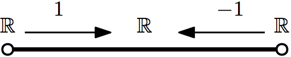
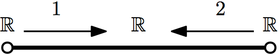
Identifying Laplacians. It’s easy to tell if an arbitrary symmetric matrix is the Laplacian of a weighted graph: check whether its diagonal is nonnegative and its row sums are zero. The problem is considerably more subtle if we want to identify sheaf Laplacians. Consider the following examples with one-dimensional stalks and two vertices:

\[\begin{bmatrix}1 & 1 \\ 1 & 1 \end{bmatrix}\]

This matrix doesn’t have zero row-sums, but it is still weakly diagonally dominant.

\[\begin{bmatrix} 1 &-2 \\\\ -2 & 4 \end{bmatrix}\]

This matrix is not even weakly diagonally dominant. It is, however ‘globally’ diagonally dominant: the sum of diagonal entries is strictly greater than the sum of absolute values of off-diagonal entries.

\[\begin{bmatrix}a^2 + b^2 & ab \\\\ ab & c^2 + d^2 \end{bmatrix}\]

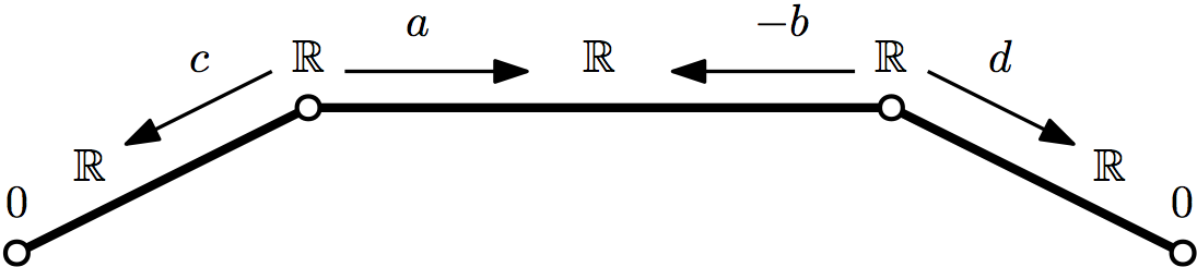
In general, a \(2\times 2\) sheaf Laplacian looks like this. We include the degenerate edges with zero stalk over one vertex for completeness and convenience. In fact, every \(2 \times 2\) symmetric positive semidefinite matrix can be written in this form. But this does not hold for larger matrices. There is, however, a necessary condition based on the \(2 \times 2\) case: To be the Laplacian of a sheaf with one-dimensional stalks, a matrix \(A\) must be totally globally diagonally dominant. That is, for every principal submatrix \(B\) of \(A\), \(B\) must be globally diagonally dominant as defined above. However, this condition is not sufficient: the matrix

\[\begin{bmatrix} 1 & 1 & \frac{1}{4} \\\\ 1 & 1 & \frac{1}{4} \\\\ \frac{1}{4} & \frac{1}{4} & 1 \end{bmatrix}\]

is not a sheaf Laplacian, but it is totally globally diagonally dominant.

When stalks are one dimensional, the question of whether \(A\) is a sheaf Laplacian is equivalent to whether there exist vectors \(v_i\) with at most two nonzero entries such that \(A = \sum_{i} v_i v_i^T\). This question of sparse decomposability seems relevant to an interesting statistics problem: Given a vector-valued random variable \(X\), when is it possible for \(X\) to have been generated by a sparse collection of independent random variables? That is, is \(X\) the sum of independent random variables, each affecting at most two coordinates of \(X\)? A necessary condition is that the covariance \(\text{Cov}(X)\) have a sparse decomposition in the sense just mentioned. This seems similar to a sparse version of principal component analysis, but current formulations of sparse PCA actually end up explaining too much variance: subtracting off all the sparse principal components leaves you with a matrix which is no longer positive semidefinite.

Applications to Systems

Dynamical Systems on Sheaves. Wherever we have a Laplacian, we want to construct heat and wave equations. These are the differential equations \(\dot x = -\alpha Lx\) and \(\ddot x = \alpha^2 L x\). The long-term behavior of the heat equation is determined by the spectrum of \(L\). In particular, the trajectory converges to the global section nearest to the initial condition. Distributed systems often use the heat equation for the graph Laplacian to achieve consensus on a value; the sheaf heat equation generalizes this concept.

The wave equation might be interesting for studying things like coupled systems of oscillators. It’s also worth noting that we can construct a Laplacian that acts on the edge stalks instead of the vertex stalks; this might be useful for other, more topological things.

The Moduli Space of Sheaves. If sheaves represent systems, then to work in the realm of possible systems, we need to study the space of sheaves. In particular, we want to ask questions like:

• How does the spectrum change as we change the sheaf?

• How to find the nearest sheaf with global sections?

• How to get a simpler sheaf that preserves important properties?

• What is a (uniformly chosen) random sheaf?

We can get coarse answers to some of these questions with spectral methods. For instance, sparsification by effective resistance works to simplify a sheaf while preserving its spectrum. Conversely, removing edges of high effective resistance pushes the sheaf closer to having global sections.

Applications to Data

Point Clouds. Sheaves have a long history of use to describe geometry. You can reasonably define a geometric space as a topological space together with a sheaf of functions on the space. So if we want to describe data geometrically, one natural approach (if you think like a pure mathematician, at least) is to try to put a sheaf on the data. This is sort of what Singer and Wu did when in their paper about vector diffusion maps and the graph connection Laplacian. They take a point cloud (assumed to be sampled from a manifold) and use local PCA to approximate the tangent space at each point, and solve the orthogonal Procrustes problem to approximate local parallel transport between tangent spaces. This fits together in an \(O(n)\)-vector bundle on the nearest-neighbor graph of the point cloud, and its associated Laplacian converges to the connection Laplacian of the manifold as the sampling density increases.

Of course, manifolds are a very special case of geometric space; in general, we don’t have a reason to assume the local dimension of our data is constant. My goal here is to investigate geometrically motivated methods that work for spaces of non-constant dimension. A simple extension of the Singer-Wu model is to simply allow the local dimension for PCA to vary, and solve a generalized orthogonal Procrustes problem to get ‘parallel transport’ maps that are rotations composed with orthogonal projections. The structural math here works out exactly as in the constant-dimension case, but it’s more difficult to interpret. What does it mean for a vector to be sent to zero under parallel transport? What continuous construction, if any, would this converge to under increasing sampling density?

A more sophisticated, better theoretically motivated construction might return to the idea of a sheaf of functions. Instead of locally approximating data by a hyperplane, as in PCA, we can get a local approximation by low-degree polynomial level sets, and construct a local space of polynomial functions for each point, hoping to patch them together via restriction maps on edges. You could look at this like a scheme, but with a finer topology than the Zariski topology.

Synchronization. The study of synchronization problems was (is being?) pioneered by Afonso Bandeira and Amit Singer. The idea behind synchronization as an approach to data analysis is that we can estimate some global information from information about local relationships. This is kind of vague. The standard example is the \(O(n)\)-synchronization problem. For concreteness, suppose we have a collection of 2D images of the same scene, but rotated differently. However, we know the relative orientations for various pairs of images. The goal for synchronization is to find a global orientation that agrees with all these pairwise rotations. A nice introduction to various sorts of synchronization problems from a very algorithmic perspective can be found in Bandeira’s notes from an MIT course in the mathematics of data science.

“Get global information from local information” is exactly the slogan for sheaf theory, so it’s natural that synchronization problems can be formulated in terms of sheaves on graphs. Every synchronization-type problem I have seen can be stated as “find an (approximate) global section for a given sheaf.” This is more general than the framework proposed by Gao, Brodski, and Mukherjee using vector bundles. The sheaf formalism, combined with spectral methods, should lead to better insights into what is possible in the world of synchronization.

There are actually a number of synchronization-like problems leveraging sheaf structure to get new information about data:

• (Synchronization) Given a sheaf, find an approximate global section or set of sections.

• (Sheaf approximation) Given maps associated to incidence relations of a cell complex, find the nearest sheaf, or find the nearest sheaf admitting global sections.

• (Clustering) Given a sheaf on a graph, find groups of connected vertices which support local sections.

• (Learning) Given cochains and frustrations (and a graph/cell complex), determine sheaf restriction maps.

Conclusion

Sheaves are a natural language for talking about many interesting problems, some of which I have outlined here. My goal is to build tools that make thinking with sheaves easier and more powerful. Spectral graph theory has powerful concepts which can be adapted to sheaves, and the more we know about the spectral theory of sheaves, the better equipped we will be to approach new problems. Conversely, it doesn’t seem unreasonable that sheaves might have something to offer back to spectral graph theory. I now have a lot of work to do!